Building a Predictive Maintenance Model
Building a Predictive Maintenance Model
Hello and welcome to another machine learning project! Today, our task is to build a predictive maintenance model for a transportation company. They have a telemetry device attached to the ECU of their vehicles and collect readings once the vehicles complete a trip OR break down in the field. Instead of checking every vehicle on a cyclical basis (once a month) we will build a model that will be able to read an observation and recommend if a vehicle will need maintenance. This will save the company money in 2 ways: reduce the amount of break-downs in the field, and increase the time needed between the cyclical vehicle check-ups.
Step 1: Exploratory Data Analysis
As always, the first step is to see what kind of data we’re working with.
data = pd.read_csv("telemetry_failures.csv")

data.head()
| date | device | failure | attribute1 | attribute2 | attribute3 | attribute4 | attribute5 | attribute6 | attribute7 | attribute8 | attribute9 | |
|---|---|---|---|---|---|---|---|---|---|---|---|---|
| 0 | 2015-01-01 | S1F01085 | 0 | 215630672 | 56 | 0 | 52 | 6 | 407438 | 0 | 0 | 7 |
| 1 | 2015-01-01 | S1F0166B | 0 | 61370680 | 0 | 3 | 0 | 6 | 403174 | 0 | 0 | 0 |
| 2 | 2015-01-01 | S1F01E6Y | 0 | 173295968 | 0 | 0 | 0 | 12 | 237394 | 0 | 0 | 0 |
| 3 | 2015-01-01 | S1F01JE0 | 0 | 79694024 | 0 | 0 | 0 | 6 | 410186 | 0 | 0 | 0 |
| 4 | 2015-01-01 | S1F01R2B | 0 | 135970480 | 0 | 0 | 0 | 15 | 313173 | 0 | 0 | 3 |
We’ll also take a look at our target variable, ‘failure’
data['failure'].value_counts()
0    124388
1       106
Name: failure, dtype: int64
As we can see, the classes are extremely imbalanced. In previous projects, we’ve had imbalanced classes and tried to work around it. In this project, I will address this issue directly using the python library imblearn.
After exploring each column in detail using value counts and pandas profiling report, I discovered each attribute is fairly abstract, so we will have to use the shape of each attribute in order to decide how to treat it.
- Based on the date column, we can tell that this data is taken from 11 months of observations
- Attributes 2, 3, 4, 7, 9 all seem to be codes since the majority of their contents are 0s.
- Attributes 1 and 6 have a fairly even spread, so we will treat those as actual numerical features.
- Attribute 7 is the same as attribute 8. Since we don’t want essentially twice the effect of that variable, we will drop it.
data.drop('attribute8', inplace=True, axis=1)
Visual EDA
Now comes the fun part of EDA. Taking a look at graphs to try and tease out trends or interesting aspects that may help with feature engineering later on. These are also useful for reporting purposes.
Time Series and Seasonality Differences
The first thing that we’ll look at is the rate of device failures across the duration of the study.
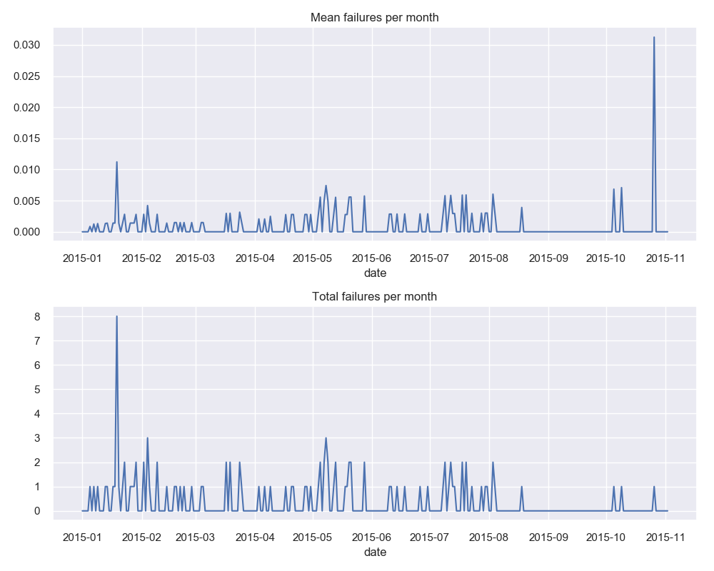
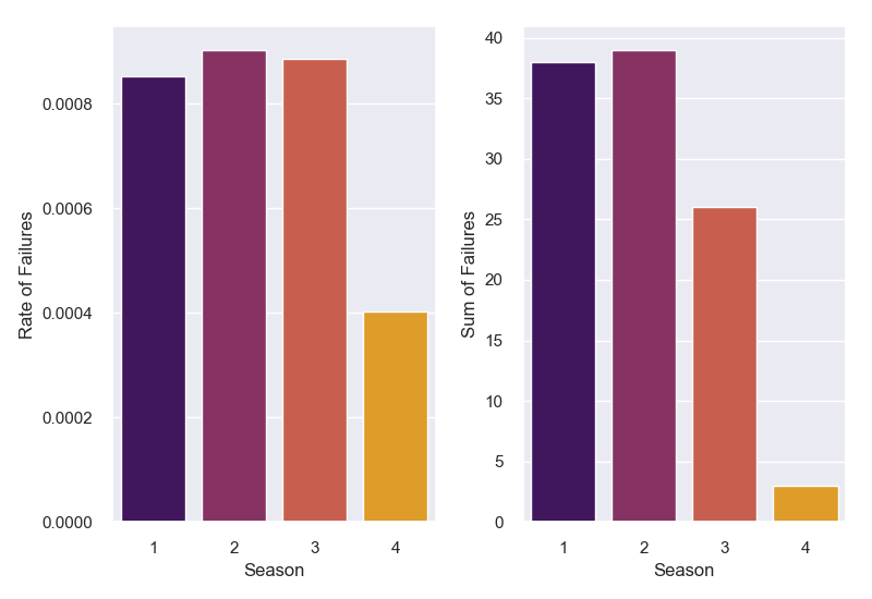
So we can see that there are more TOTAL failures in January 2015, but the overall RATE of failure (failure/ number of shipments) had a larger spike at the end of October 2015, around 3% failure rate. As we can see below, this means that there are some seasonality differences of shipments.
General Distribution Comparisons
Since our target is not normally distributed, I wanted to take a closer look at how close it is to a Poisson distribution, which is used when you know how many events to expect in a certain time frame, but the time between events is independent.
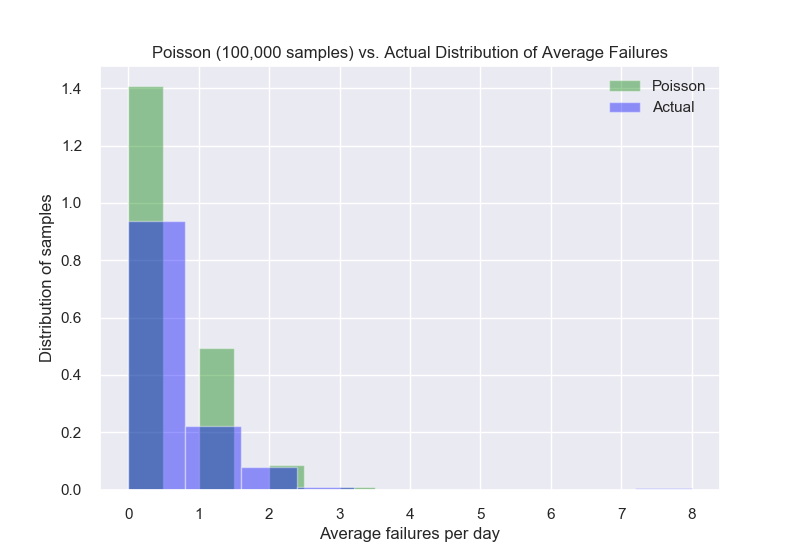
We can see it follows the same trend of a Poisson distribution but of course it’s not perfect.
Groupby Graphs
From here I wanted to take a closer look at how failed device features differed from working device features.
failed_devices = vis_data[vis_data['failure'] == 1]
working_devices = vis_data[vis_data['failure'] == 0]
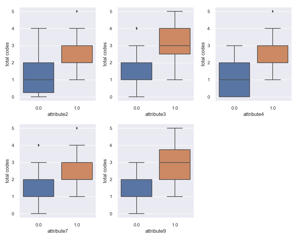
After taking a sum of the categorical codes that we specified earlier, we can see if certain codes have ‘comorbidity’, the presence of an attribute means a higher chance of other attributes also being present. So we would expect if there is no comorbidity, the difference between the presence of an attribute would be exactly 1 ‘total code’.
After looking at this, I wanted to see if there was an effect of seasonality as well. The graph below is the same as above with an extra variable (season) also shown.
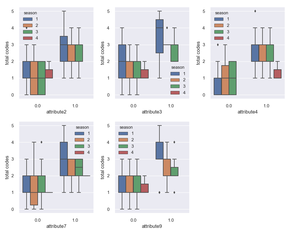
This graph is useful for showing the seasonality of each attribute in failed devices. For example, we see that attribute 2, 3, and 9 rarely occur in the fall. This could be due to the low sample size of those fall failures.
Ok, we have a pretty good sense of the data now, we can start really drilling down and building a DataFrame to model.
Groupbys and Feature Engineering
The first thing that we can do is add a variable for seasonality.
#Adding the season variable
data['date'] = pd.to_datetime(data['date'])
data['season'] = data['date'].apply(lambda dt: (dt.month%12 + 3)//3)
data['season'] = data['season'].astype(str)
The next thing that we’ll do is identify the devices that went out after failure. Of the 106 devices that failed, there were 5 that went on another trip after their failure date.
I accomplished this by grouping the devices by failure/non-failure, tagging the max date they went out, and then re-combining and comparing those DataFrames
| attribute1_fail | attribute2_fail | attribute3_fail | attribute4_fail | attribute5_fail | attribute6_fail | attribute7_fail | attribute9_fail | failure_date | |
|---|---|---|---|---|---|---|---|---|---|
| device | |||||||||
| S1F023H2 | 64499464 | 0 | 0 | 1 | 19 | 514661 | 16 | 3 | 2015-01-19 |
| S1F03YZM | 110199904 | 240 | 0 | 0 | 8 | 294852 | 0 | 0 | 2015-08-03 |
| S1F09DZQ | 77351504 | 2304 | 0 | 3 | 7 | 418563 | 0 | 2 | 2015-07-18 |
| S1F0CTDN | 184069720 | 528 | 0 | 4 | 9 | 387871 | 32 | 3 | 2015-01-07 |
| S1F0DSTY | 97170872 | 2576 | 0 | 60 | 12 | 462175 | 0 | 0 | 2015-02-14 |
| S1F0F4EB | 243261216 | 0 | 0 | 0 | 10 | 255731 | 0 | 3 | 2015-05-07 |
| S1F0GG8X | 54292264 | 64736 | 0 | 160 | 11 | 192179 | 0 | 2 | 2015-01-18 |
| S1F0GJW3 | 83874704 | 2144 | 0 | 401 | 9 | 229593 | 16 | 0 | 2015-03-17 |
| S1F0GKFX | 121900592 | 0 | 0 | 18 | 65 | 246719 | 0 | 0 | 2015-04-27 |
| S1F0GKL6 | 160459104 | 0 | 0 | 2 | 90 | 249366 | 0 | 0 | 2015-05-13 |
#Step 2: Building the Model
Creating the Model DataFrame
device_group = data.groupby('device').agg({'failure': 'sum', 'attribute1' : 'mean', 'attribute2': ['min','max'],
                                           'attribute3':['min','max'], 'attribute4': ['min','max'], 'attribute5': 'mean',
                                           'attribute6': 'mean', 'attribute7': ['min','max'], 'attribute9':['min','max', 'count']})

device_columns = ['failure', 'attribute1mean','attribute2min','attribute2max', 'attribute3min','attribute3max',
                  'attribute4min','attribute4max', 'attribute5mean', 'attribute6mean', 'attribute7min','attribute7max',
                  'attribute9min','attribute9max', 'days working']

device_group = pd.DataFrame(device_group, index = device_group.index)
device_group.columns = device_columns

#Creating the sent_after_failure column
sent_after_failure = ['S1F0GPFZ', 'S1F136J0', 'W1F0KCP2', 'W1F0M35B', 'W1F11ZG9']

device_group['sent_after_failure'] = 0
device_group.loc[sent_after_failure, 'sent_after_failure'] = 1
From here, I separate the features and target columns, and create a user-defined function to finish the pre-processing (dummies on all the object columns).
Modeling and Pipelines
In many projects, the target variable will be unbalanced by necessity. I would hope there are a much higher amount of devices that did NOT fail in comparison to devices that do fail. Or an example from a previous project: more people will repay a loan than default on a loan.
I will go over one technique to solve this problem of class imbalance. I will also show a bit of sklearn’s Pipeline function, which is useful for comparing different models, hyperparameters, and balancing techniques.
#imports needed
from imblearn.over_sampling import SMOTE
from imblearn.pipeline import make_pipeline

from sklearn.ensemble import GradientBoostingClassifier, RandomForestClassifier

from sklearn.metrics import accuracy_score, precision_score, f1_score, recall_score
from sklearn.model_selection import train_test_split
from sklearn.metrics import classification_report
#Instanciate SMOTE, Random Forest Classifier, and Gradient Boost Classifier

sm = SMOTE(sampling_strategy= 'auto', random_state=42)
sm2 = SMOTE(sampling_strategy= 1 , random_state=42)


r = RandomForestClassifier()
gbc = GradientBoostingClassifier()
gbc2 = GradientBoostingClassifier(learning_rate= 1.5, n_estimators= 40, max_depth= 12, random_state=42)
l = LogisticRegression()


rf_pipeline = make_pipeline(sm, r)

rf_pipeline2 = make_pipeline(sm2, r)

gbc_pipeline = make_pipeline(sm, gbc)

gbc_pipeline2 = make_pipeline(sm2, gbc)

gbc_pipeline3 = make_pipeline(sm2, gbc2)


classes = ["Working Device", "Failed Device"] #Needed for the visualizers
Synthetic Minority Over-sampling Technique (SMOTE) is a re-sampling technique that synthetically generates data points that are similar to the minority class (failed devices). The ratio of samples in the minority vs. majority class can be manipulated using the sampling_strategy argument.
In addition to that, I wanted to compare the difference between Random Forest and Gradient Boosting models, since they performed the best in my user defined function that quickly compares models.
I created 5 pipelines and compared metrics between them, an example of the best pipeline (gbc_pipeline2) is shown below.
#Train/Test/Split
X_train, X_test, y_train, y_test = train_test_split(features, target, test_size = .3,
stratify=target, random_state = 42)

# Pipeline here
gbc_pipeline2.fit(X_train, y_train)

#Sklearn Classification report
y_pred = gbc_pipeline2.predict(X_test)

print(classification_report(y_test, y_pred))
Then we run each pipeline through Yellowbrick’s classification report, confusion matrix, and ROCAUC functionalities.
#YellowBrick Classification report

visualizer = ClassificationReport(gbc_pipeline2, classes=classes)
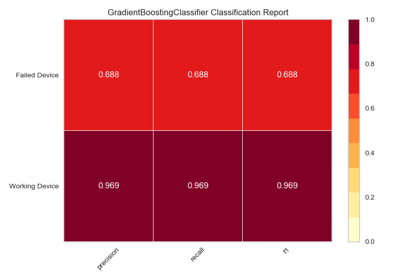
Since our objective is to predict which devices will fail on the next trip, the metric we want to focus on here is the Recall for failed devices.
#Confusion Matrix
cm = ConfusionMatrix(gbc_pipeline2, classes=[0,1])

In the confusion matrix, we can see that we correctly classify 22/32 failed devices. This is useful for getting a sense of how our algorithm would classify in a real study and spread of the data.
#Yellowbrick ROC/AUC

visualizer = ROCAUC(gbc_pipeline2, classes=classes)
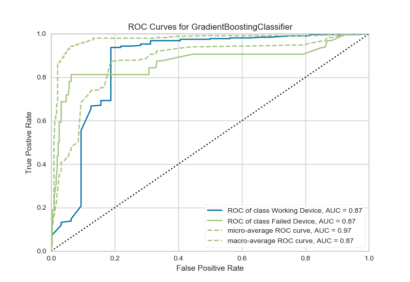
The ROC AUC curve shows how well the algorithm can distinguish between when a failed device and functioning device. That means our model is 87% sure that it can distinguish between the classes.
Conclusion
# Final test with whole dataset:

#Confusion Matrix
cm = ConfusionMatrix(gbc_pipeline2, classes=[0,1])

# Fit fits the passed model.
cm.fit(X_train, y_train)
cm.score(features, target)
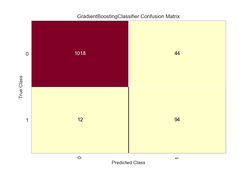
Our goal was to create a machine learning model to predict if a vehicle would fail on it’s next trip based on data from a telemetry device. Using this model, the company can now catch 94 out of every 106 devices that fails . This will increase the company’s rate of successfully completed trips, increasing their revenue in multiple ways (saving towing costs, better customer relations).
Thank you for taking the time to read through this project and if you have any questions or concerns please dont hesitate to reach out via email!

Hello! Welcome to my site. This is where I showcase my completed projects.