Kaggle Competition Predicting House Prices
Predicting House Prices - Kaggle Competition
Hello again! For this project I will be doing a Kaggle competition, the Ames Housing dataset. This is an advanced regression problem that requires careful data cleaning, attentive feature engineering, and LOTS of time spent analyzing features. As with most of my projects, I will be showing the clean, pretty copy of my work.
The data itself comes with the training and test sets (test set not containing the target variable - price). We need to combine them in order to do the same transformations on the features, then at the last second we will split them again. There are 80 features that we need to sift through, many of them relating to a similar theme (basement/garage/outdoor space).
df.isnull().sum()

1stFlrSF            0
2ndFlrSF            0
3SsnPorch           0
Alley            2721
BedroomAbvGr        0
BldgType            0
BsmtCond           82
BsmtExposure       82
BsmtFinSF1          1
BsmtFinSF2          1
BsmtFinType1       79
BsmtFinType2       80
BsmtFullBath        2
BsmtHalfBath        2
BsmtQual           81
BsmtUnfSF           1
CentralAir          0
Condition1          0
Condition2          0
Electrical          1
EnclosedPorch       0
ExterCond           0
ExterQual           0
Exterior1st         1
Exterior2nd         1
Fence            2348
FireplaceQu      1420
Fireplaces          0
Foundation          0
FullBath            0
                 ...
LotShape            0
LowQualFinSF        0
MSSubClass          0
MSZoning            4
MasVnrArea         23
MasVnrType         24
MiscFeature      2814
MiscVal             0
MoSold              0
Neighborhood        0
OpenPorchSF         0
OverallCond         0
OverallQual         0
PavedDrive          0
PoolArea            0
PoolQC           2909
RoofMatl            0
RoofStyle           0
SaleCondition       0
SalePrice        1459
SaleType            1
ScreenPorch         0
Street              0
TotRmsAbvGrd        0
TotalBsmtSF         1
Utilities           2
WoodDeckSF          0
YearBuilt           0
YearRemodAdd        0
YrSold              0
Length: 81, dtype: int64
Section 1: Data Cleaning
Problem:
- Many null values in many columns
Solution:
- Fill values using data documentation, fill with median(numerical), mode(categorical)
Problem:
- String rankings from Excellent to Poor/Na
Solution:
- Replace with numerical rankings so we dont have to get dummies on so many columns
#Feature Transformation (Changing string to numerical rankings)
df.replace(['Ex', 'Gd', 'TA', 'Fa', 'Po', 'NA'], [5, 4, 3, 2, 1, 0], inplace = True)

#In documentation it says that BsmtQual corresponds to height
df['BsmtHeight'] = df['BsmtQual']

df['BsmtExposure'].replace(['Gd', 'Av', 'Mn', 'No'], [3, 2, 1, 0], inplace = True)
df['CentralAir'].replace(['Y', 'N'], [1,0], inplace = True)
df['GarageFinish'] = df['GarageFinish'].replace(["Fin", "RFn", "Unf", 'NA'], [3,2,1,0])
df['PavedStreet'] = df['Street'].replace(['Pave', 'Grvl'], [1,0])
df['LandSlope'] = df['LandSlope'].replace(["Gtl", "Mod", "Sev"], (3, 2, 1))

#Filling nulls according to the feature notes in Kaggle, or filling with most common value

df['MasVnrType'] = df['MasVnrType'].fillna('None')
df['MasVnrArea'] = df['MasVnrArea'].fillna(0)

df['Exterior1st'] = df['Exterior1st'].fillna('VinylSd')
df['Exterior2nd'] = df['Exterior2nd'].fillna('VinylSd')

df['BsmtHeight'] = df['BsmtHeight'].fillna('NA')
df['BsmtCond'] = df['BsmtCond'].fillna('NA')
df['BsmtExposure'] = df['BsmtExposure'].fillna('NA')
df['BsmtFullBath'] = df['BsmtFullBath'].fillna(0)
df['BsmtHalfBath'] = df['BsmtHalfBath'].fillna(0)
df['TotalBsmtSF'] = df['TotalBsmtSF'].fillna(0)

df['GarageType'] = df['GarageType'].fillna('NA')
df['GarageYrBlt'] = df['GarageYrBlt'].fillna(df['YearBuilt'])
df['GarageCars'] = df['GarageCars'].fillna(0)


df['GarageCond'] = df['GarageCond'].fillna(0)
df['GarageFinish'] = df['GarageFinish'].fillna('NA')
df["FireplaceQu"].fillna(0, inplace = True)
df['MiscFeature'].fillna('None', inplace = True)

df['PoolQC'] = df['PoolQC'].fillna('None')
df['Alley'] = df['Alley'].fillna('None')

df['Electrical'] = df['Electrical'].fillna('SBrkr')
df['KitchenQual'] = df['KitchenQual'].fillna(3)
df['Functional'] = df['Functional'].fillna('Typ')
df['Utilities'] = df['Utilities'].fillna('AllPub')
df['SaleType'] = df['SaleType'].fillna('WD')
df['MSZoning'] = df['MSZoning'].fillna('RL')
df['Fence'] = df['Fence'].fillna(0)

df['LotFrontage'] = df.groupby('Neighborhood')['LotFrontage'].transform(lambda x: x.fillna(x.median()))

df.replace(['Ex', 'Gd', 'TA', 'Fa', 'Po', 'NA'], [5, 4, 3, 2, 1, 0], inplace = True)
Section 2: Primary Feature Engineering
Now that we’ve cleaned up the data feature by feature, we can combine some unnecessary or extraneous features.
#Create an overall score for the exterior
df['OverallExterScore'] = df['ExterQual'] + df['ExterCond']

#combining basement bathrooms
df['BsmtBathTotal'] = df['BsmtHalfBath'] + df['BsmtFullBath']

#Create a basement completion rating
df['BsmtCompletion'] = np.where(df['BsmtFinType1'] != 'Unf', 1, 0)

#Combining bathrooms
df['HalfBath'] = df['HalfBath'] * 0.5
df['Bathrooms'] = df['HalfBath'] + df['FullBath']

#Combining Outdoor Living Features
df['OutdoorLivingSqft'] = (df['WoodDeckSF'] + df['OpenPorchSF'] + df['EnclosedPorch'] +
                                  df['3SsnPorch'] + df['ScreenPorch'])

#Combining Date Sold Features
df['TimeSold'] = df.apply(lambda x: dt.date(x['YrSold'], x['MoSold'], 1), axis=1)

#Recently Remodeled Feature
df['RecentRemodel'] = ((df['YearRemodAdd'] > (df['YearBuilt'] + 25)))

#Changing MSSubclass to catagorical:
df['MSSubClass'] = df['MSSubClass'].astype(str)
There are also 4 outliers for GrLivArea that need to be dropped in order to show the model a better linear relationship.
Section 3: Graphs of Data relationships
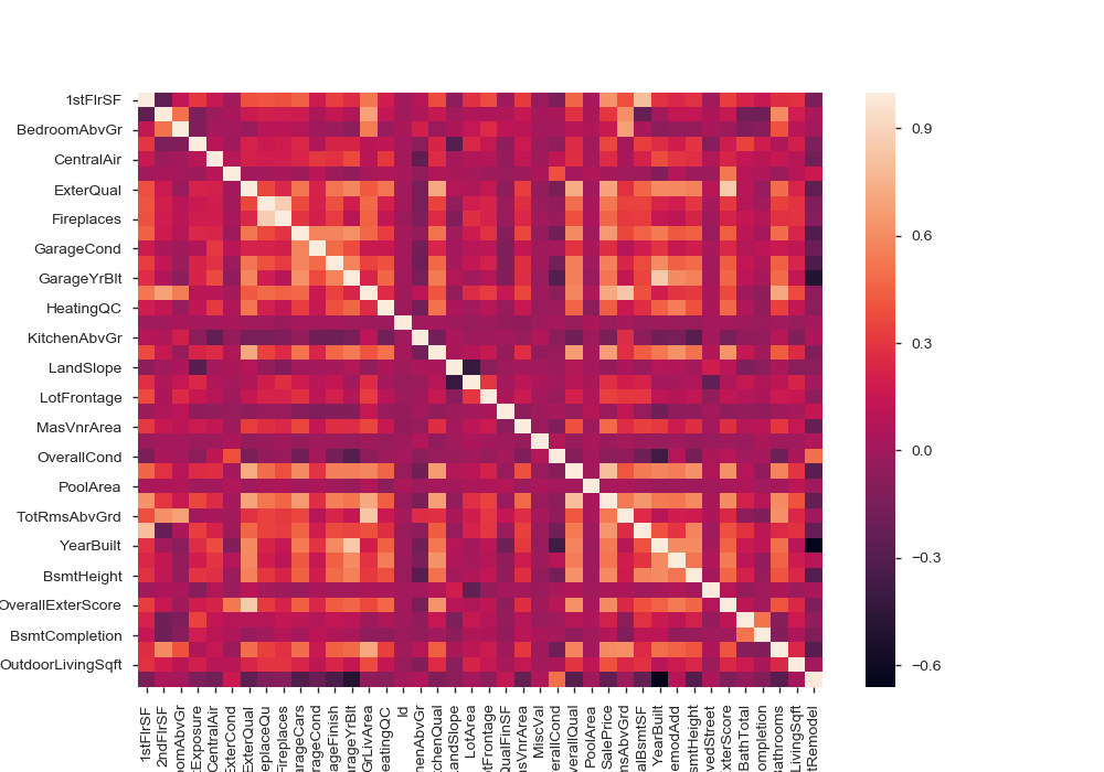
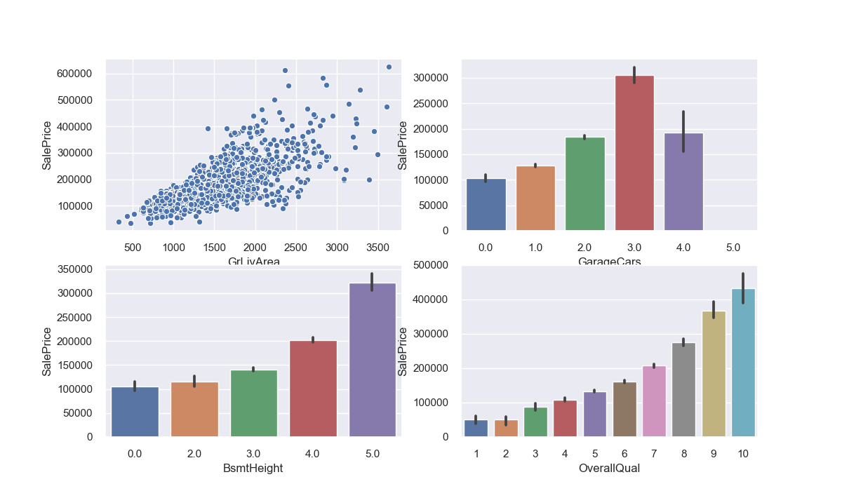
Let’s take a break from the coding bit and see what we’ve actually done with our data. We can take a look at the heatmap of the correlations between variables, and then drill down into the ones that have the most interesting relationship with Sale Price.
We can also take a moment to analyze the range and skew of Sale Price.
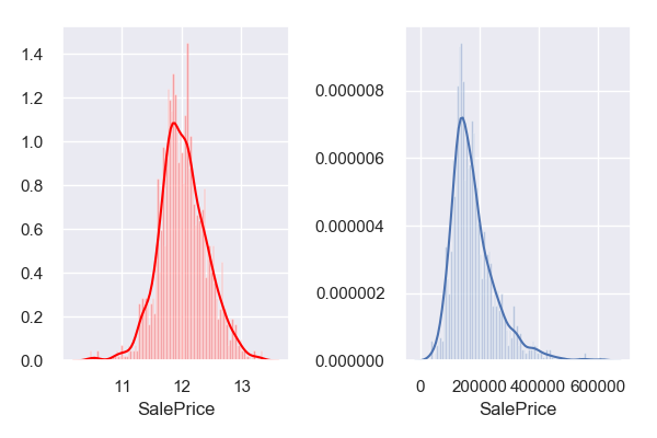
We can see that the log of sale price is statistically more normal, so using that would be much easier for our model. This leads us to some more feature engineering!
Section 4: Further Feature Engineering
Here we will separate our numerical and categorical (string) features. We check the numerical ones for skew, and if they are over a certain threshold, we use the log of that feature. We also take this opportunity to get dummies on our categoricals, and re-combine the data.
#Splitting numerical and object columns off
numerical_features = df_train.select_dtypes(exclude='object').columns
object_features = df_train.select_dtypes(include='object').columns

train_num = df_train[numerical_features]
train_cat = df_train[object_features]

#Checking and adjusting for skew:
skewness = train_num.apply(lambda x: skew(x))
skewness = skewness[abs(skewness) > 0.5]
#remove the Boolean and negative values
skewness.drop(['RecentRemodel'] ,inplace = True)

skewed_features = skewness.index

train_num[skewed_features] = np.log1p(train_num[skewed_features])

#Re-join numerical and catagorical
df_train = pd.concat([train_num, train_cat], axis = 1)
df_train['RecentRemodel'] = df['RecentRemodel']

features = df_train.iloc[:1455]
test_features = df_train.iloc[1455:]

#Use the log of our target column
target = np.log1p(df.loc[:1459, 'SalePrice'])
#target = training['SalePrice']
After properly separating our training and test sets out, we focus on the training set for modelling. We use sklearn’s train_test_split and assess which regression technique will be best fit for the problem.
R^2 train R^2 test RMSE train RMSE test
Linear Regression 0.936612 0.886556 0.098704 0.135246
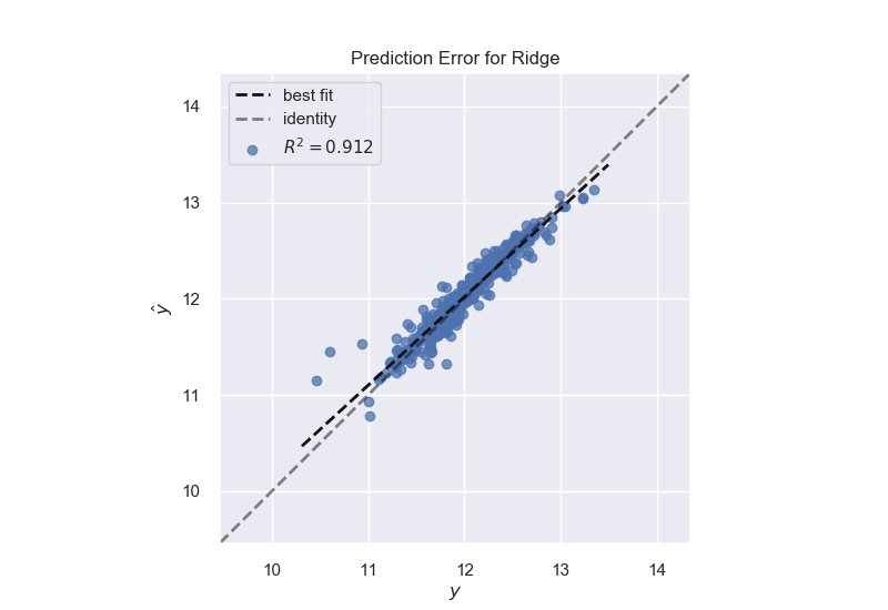
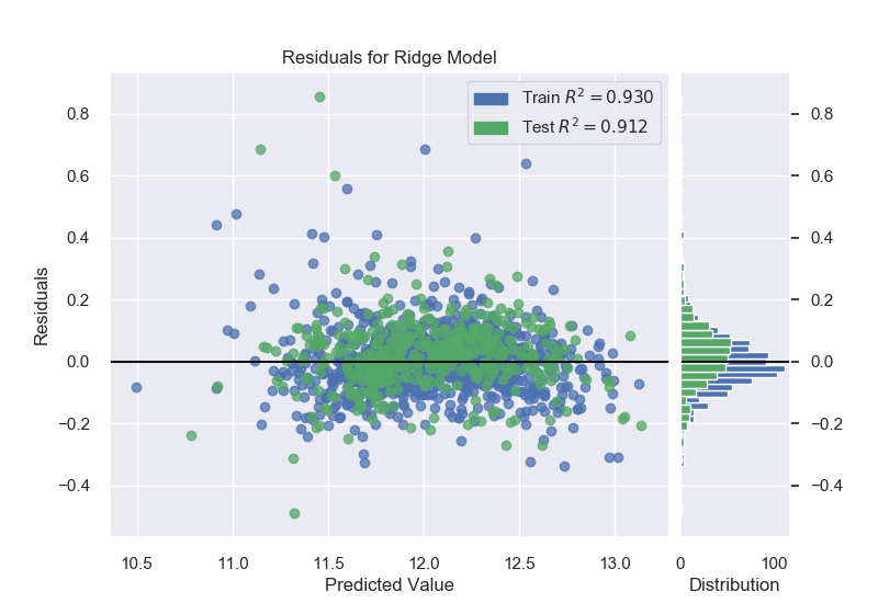
Ridge 0.929799 0.912495 0.103873 0.118782
Lasso 0.000000 -0.013611 0.392042 0.404268
Elastic Net 0.000000 -0.013611 0.392042 0.404268
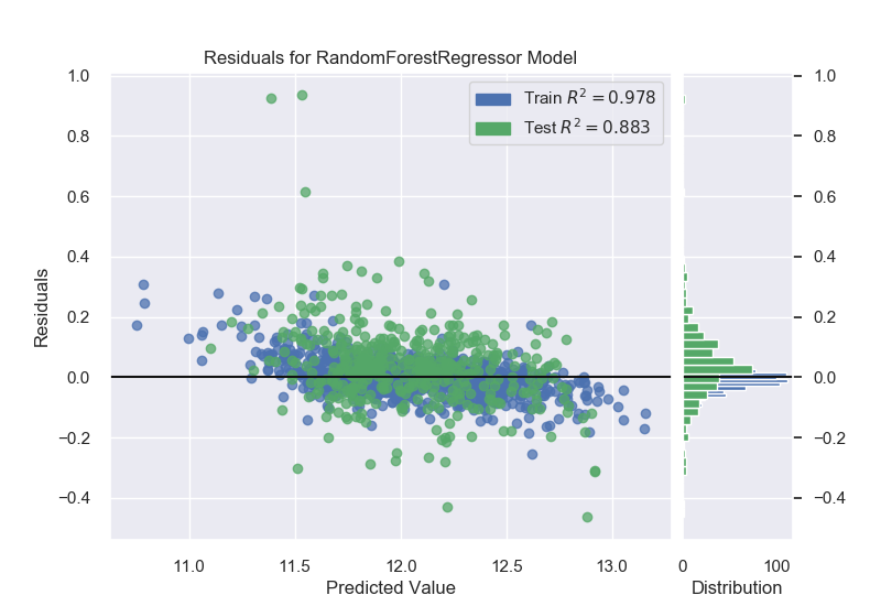
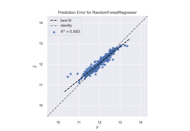
Random Forest 0.978379 0.883046 0.057646 0.137322
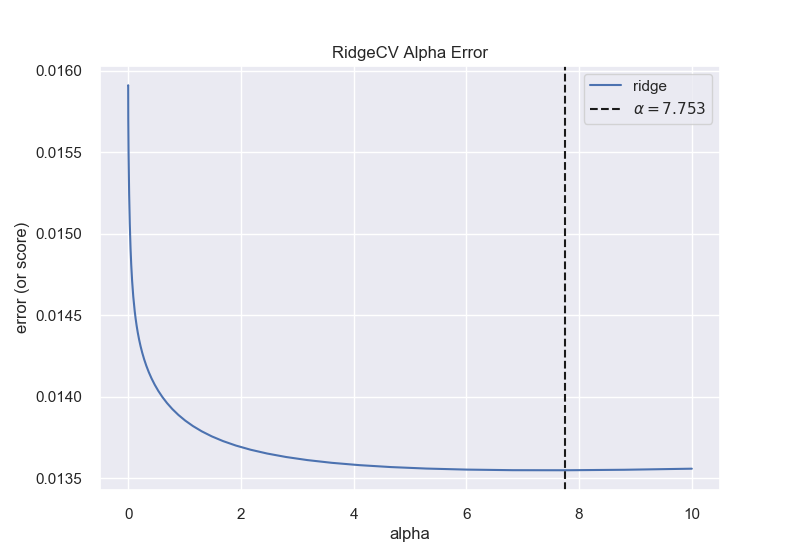
Since Ridge and Random Forest perform the best for this problem, we will be focusing on those. We will use yellowbrick alpha selector to tune Ridge and a grid search process to tune the Random Forest.
Ridge Model:
Random Forest Model:
I chose to stay with the Ridge Regressor to predict and submit to Kaggle. After using the predict statement, I made sure to transform the Sale Price back to its original scale with np.expm1.
Using this approach got me top 36% on the Kaggle leader boards. I could add some further depth and increase my score if I used model stacking for higher price ranges where the Ridge model starts to deviate, but that will not be covered in this post at this time. Thank you for taking the time to look at my work and as always please reach out to me if you see any errors or have any questions!

Hello! Welcome to my site. This is where I showcase my completed projects.