Predicting Loan Repayment

The Business case for this problem is that a bank wants us to generate a list of questions for them to ask potential customers in order to predict whether or not their loans will be repaid.

#import libraries
import pandas as pd
import numpy as np
import matplotlib.pyplot as plt
import matplotlib.image as mpimg
import seaborn as sns

from sklearn.ensemble import GradientBoostingClassifier, RandomForestClassifier
from sklearn.ensemble import RandomForestRegressor
from sklearn.tree import DecisionTreeClassifier
from sklearn.linear_model import LogisticRegression
from sklearn.model_selection import train_test_split
from sklearn.metrics import accuracy_score, precision_score, f1_score, recall_score

Section 1: Introduction and Basic EDA

The data that we have for this problem is intentionally problem-ridden, so there is much cleaning to be done. Our target variable this time is Loan Status, so we will be sure to keep an eye out for how the other features have an effect on this.

There are 6 columns with null values that we will have to handle at some point. Lets take a look at their values first. Some we will look at value counts, some we will look at nunique depending on what I think we will end up doing to them.

Section 2: Data Cleaning:

After looking through all the variables and their types, below is a list of things that need to be fixed. I will briefly go over how I solved each issue.

2a:Dropping duplicate Entries

2b:Some values in the Credit Score column are multiplied by 10.

2c:Monthly Debt column contains ‘$’ and ‘,’ symbols.

2d:Convert our target column, Loan Status, to a binary.

2e:Current Loan Amount has many outlier values.

2f:The Purpose column has 2 values indicating ‘Other’.

2g:Maximum Open Credit has 2 different ‘0’ values, and is an object type when it should be float.

2h:Home Ownership has 2 values that are essentially the same: ‘HaveMortgage’ and ‘Home Mortgage’

2i:Years in Current Job has about 10,000 missing values.

2j:Bankruptcies and Tax Liens have some missing values.

2k:Handling 61,000 missing values in Credit Score and Annual Income.

2a: Drop Duplicate Entries

Some of these values are not just duplicates, but triplets or quadruplets, so we have to sort by LoanID when we drop them.

loans.drop_duplicates(subset='Loan ID', inplace = True)

2b: Fix Erronious Values in Credit Score

We can fix this with a simple list comprehension

loans['Credit Score'] = [score/10 if score > 800 for score in loans['Credit Score']]

loans['Credit Score'].describe()

2c: Converting Loan Status to a Binary

loans['Loan Status'].value_counts()

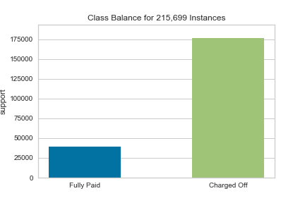
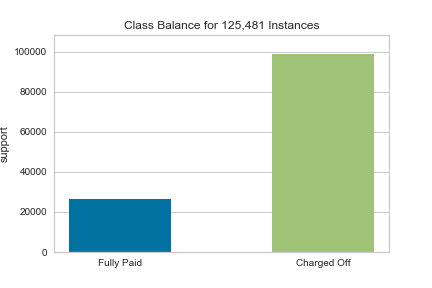
Here we see that our target variable is imbalanced (there are 176,000 fully paid loans and 40,000 unpaid loans). This will create some inaccuracy in our model later. It can be (mostly)solved with undersampling the fully paid loans, or oversampling the unpaid loans. I will not be covering this approach at the current time, but I will be testing a couple different models to see how the imbalance affects our predictions.

loans['Loan Status'].replace(['Fully Paid', 'Charged Off'], [1,0], inplace = True)

2d: Strip Monthly Debt

Currently Monthly Debt has a dollar sign in the front and a comma separating the thousands place.

loans['Monthly Debt'].replace(to_replace=['\$',','],value=["",""],regex=True, inplace=True)
loans['Monthly Debt'] = loans['Monthly Debt'].astype(float)

I also noticed in our describe statement that the max monthly debt is a massive outlier at $23,000. This would unnecessarily skew our model, so we’ll remove this point.

There are also 215 people with a Monthly Payment of $0. This doesn’t seem right but I’m hesitant to drop so many rows when there is nothing wrong with the rest of the columns.

2e: Fixing Current Loan Amount

There are about 35,000 Current Loan Amounts that are misentered as 99999999.

All of these misentered loans are also in one group of our target variable (Fully Paid). This is our class with many more observations. I will be doing 3 methods to fill these values: -Imputing with the mean -Imputing with Random Forest Regressor -Drop these rows in order to attempt to balance the classes

In this specific section, I will impute with the mean.

nol_filled_loans= non_outlier_loan[non_outlier_loan['Loan Status'] == 1]
nol_filled_loans_mean = nol_filled_loans['Current Loan Amount'].mean()

#fill with the mean:
nol_mean = non_outlier_loan['Current Loan Amount'].mean()
loans['Current Loan Amount'].replace(99999999.0, value = nol_filled_loans_mean, inplace=True)

If you look in the KDE graphs in Section 4, you will see that filling with the mean skews the paid loans quite a bit.

2f: Fixing the Purpose Column

This one is a quick fix, there are just two different values for ‘Other’

loans['Purpose'] = loans['Purpose'].str.replace('other', 'Other')
loans['Purpose'].value_counts()

2g: Fixing Maximum Open Credit

This one is similar, there are two different values for 0, and some odd ‘#VALUE!’…. values.

loans['Maximum Open Credit'] = loans['Maximum Open Credit'].replace(to_replace = 0, value = '0')

loans['Maximum Open Credit'].replace(to_replace = '#VALUE!', value = '0', inplace=True)

loans['Maximum Open Credit'] = loans['Maximum Open Credit'].astype(int)

2h: Fixing Home Ownership

Here we can see a similar case, there are two values that seem to have the same meaning.

loans['Home Ownership'].value_counts()

loans['Home Ownership'].replace(to_replace = 'HaveMortgage', value = 'Home Mortgage', inplace=True)
loans['Home Ownership'].value_counts()

2i: Filling Years in Current Job

There are about 9,000 nulls in the Years in Current Job column.

loans['Years in current job'].isnull().sum()

loans['Years in current job'].value_counts()

We are going to fill with ‘0 years’ because the only thing that distinguishes the null values from non is that their Annual Income is much lower. See graph in Section 4 that shows this.

loans['Years in current job'].fillna(value='0 years', inplace = True)

2j: Filling Bankruptcies and Tax Liens

There are only a few nulls in these categories, and 0 is an extremely common value, so filling with 0 shouldn’t be a problem.

loans['Bankruptcies'].fillna(value=0, inplace = True)
loans['Tax Liens'].fillna(value=0, inplace = True)

2k: Handling Null Values in Annual Income and Credit Score

Here we will be filling the 60,000 null values in each of these columns using regression. I will also be segmenting each DataFrame so that we have 4 different options when modeling:

• “Basic model”: Null values in Credit Score + Annual Income dropped, Current Loan Amount imputed with mean
• Null values in Credit Score + Annual Income filled with regression, CLA imputed w/ mean
• Null values in Credit Score + Annual Income dropped, CLA filled with regression
• “Class Balanced”: Null Values in Credit Score + Annual Income dropped, CLA dropped

First we will define a function to prep each DataFrame. This will be useful to prep the null DataFrame and then used again to fill a copy of the original dataframe with the predicted values.

We will assess the R^2 score and root mean squared error of each model: Linear Regression, Ridge, Lasso, and Random Forest Regressor to see which best fits. Spoiler alert: Random Forest works best for Credit Score and Current Loan Amount, and Linear Regression works best for Annual Income.

def regressprep(df):
    """Prepare a DataFrame for the Regression fill"""

    df.drop(['Customer ID', 'Loan ID'], axis=1, inplace = True)

    #Splitting numerical and object columns off
    numerical_features = df.select_dtypes(exclude='object').columns
    object_features = df.select_dtypes(include='object').columns

    train_num = df[numerical_features]
    train_cat = df[object_features]

    #Get Dummies on Object columns
    train_cat = pd.get_dummies(train_cat, drop_first= True)

    df = pd.concat([train_num, train_cat], axis = 1)
    return df

After doing quite a bit of messy work, we have the 4 DataFrames set up for some feature engineering.

Section 3: Feature Engineering

df_list = [loans, df_credit_income_imputed, df_current_loans_imputed, balanced_loans]

We will create a list of our frames in order to perform the same processes on each. Some features that I thought may be useful with the given data are:

* "Major Issues": (Tax Liens + Bankruptcies + Credit Problems)
* "Debt to Income ratio": ('Monthly Debt' / (('Annual Income' +1) / 12))
* "Current Available Balance": ('Max Open Credit' -'Current Credit Balance')

Section 4: Graphs

Before modeling, here are some graphs to show the reasoning behind the data cleaning and compare the difference between our DataFrames.

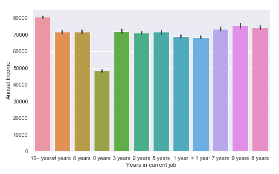
This graph shows why we created a new class ‘0 Years’ for the nulls in Years in Current Job. I could have also called this class ‘Unemployed’, but I wanted to keep with the naming convention of the column.

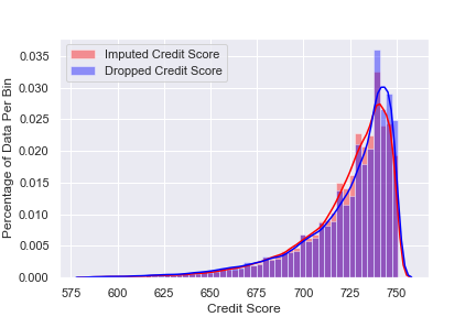
Here you can see the distribution of Credit Score for our basic model vs. imputed with random forest regressor. The imputed values seem to be a bit more evenly distributed.

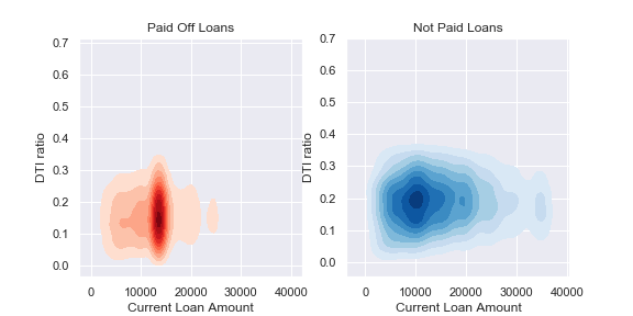
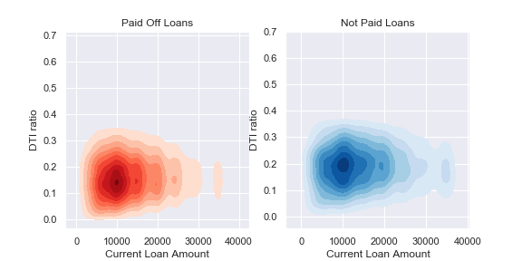
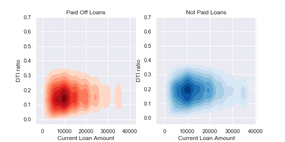
These graphs compare the differences in imputing Current Loan Amount, graphed against Debt to income ratio and Loan Status. We can see imputing with the mean gives a much more skewed distribution for that class, so that might give our model some trouble generalizing to new data.

Section 5: Modeling

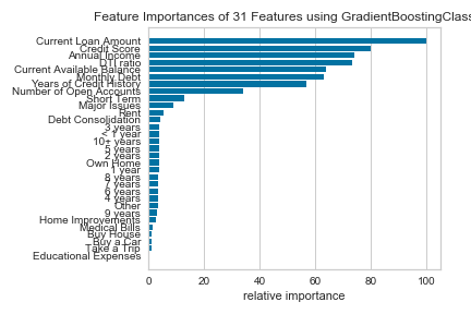
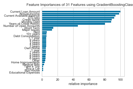
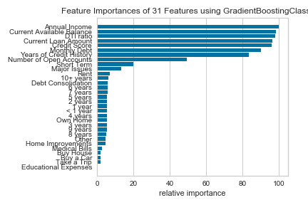
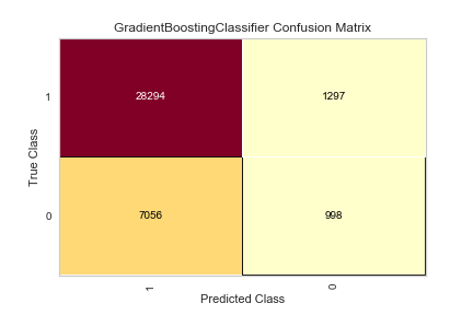
This was an extremely time consuming process, but luckily much can be explained by graphs. I will list each model and 3 figures to show assessment: feature importance, class imbalance, and the confusion matrix. The models have been tuned based on the basic dataframe (tuning each one would be far too time consuming).

Basic Model:

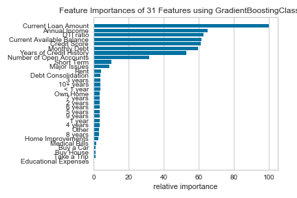
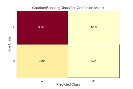
You can see how the class imbalance plays a large part in the model. While the overall accuracy is not bad, the algorithm over-predicts that people WILL pay their loans, when people are actually NOT going to pay their loans.

Credit Score and Annual Income Imputed with Regression:

Current Loan Amount Imputed with Regression:

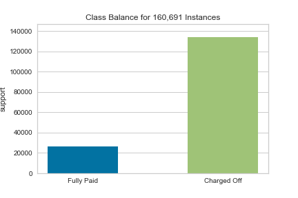
“Class Balanced” by dropping Current Loan Amount:

Still only 44% accurate in correctly predicting if people will NOT pay their loans, only 1% better than the basic model. As mentioned before, this may be fixed with undersampling (the Fully Paid loans) or oversampling (the Charged Off loans).

Conclusion

Since our assignment was to create questions for the bank to ask a potential customer, we base our questions below on the highest feature importances from our best model above.

1. What is the customer’s income?
2. How much are they going to pay per month?
3. How much is their “available balance”?
4. What is their Credit Score, and how many years of credit history do they have?
5. How many open accounts do they currently have?

Thank you for taking the time to read through this project! If you have any questions or would like to see the full Jupyter notebooks, please let me know.

Graphs made by using matplotlib, seaborn, and yellowbrick.