Anticipating Utility Site Disruptions

Our business question in this situation is that a Utility company wants to predict their site disruptions in order to minimize the amount of time that their service is down. My boss has come to me and asked me to generate a report every morning in order to preemptively predict these disruptions so that she can send out service technicians to their first location in the morning.

Each service station has a fault severity of 0 (no issues), 1 (minor issues), or 2 (major issue). The other data that are given to us are fairly abstract in nature, but we know each observation is a single instance of a service check on the station.

#import libraries
import pandas as pd
import numpy as np
import matplotlib.pyplot as plt
import seaborn as sns
from functools import reduce


from sklearn.ensemble import GradientBoostingClassifier, RandomForestClassifier
from sklearn.tree import DecisionTreeClassifier
from sklearn.linear_model import LogisticRegression
from sklearn.model_selection import train_test_split
from sklearn.metrics import accuracy_score, precision_score, f1_score, recall_score

After importing the libraries, we read in the data, which is given to us in 4 different tables. After taking a look at each one, we clean them up enough to combine together

df_list = [event_tb, log_tb, resource_tb, severity_tb, train_tb]

for item in df_list:
    print(item.head())

     id     event_type
0  6597  event_type 11
1  8011  event_type 15
2  2597  event_type 15
3  5022  event_type 15
4  5022  event_type 11
     id  log_feature  volume
0  6597   feature 68       6
1  8011   feature 68       7
2  2597   feature 68       1
3  5022  feature 172       2
4  5022   feature 56       1
     id    resource_type
0  6597  resource_type 8
1  8011  resource_type 8
2  2597  resource_type 8
3  5022  resource_type 8
4  6852  resource_type 8
     id    severity_type
0  6597  severity_type 2
1  8011  severity_type 2
2  2597  severity_type 2
3  5022  severity_type 1
4  6852  severity_type 1
      id      location  fault_severity
0  14121  location 118               1
1   9320   location 91               0
2  14394  location 152               1
3   8218  location 931               1
4  14804  location 120               0

#Merge the dataframes together
df = reduce((lambda df1, df2: pd.merge(df1, df2, on='id')), df_list)

df.info()

<class 'pandas.core.frame.DataFrame'>
Int64Index: 61839 entries, 0 to 61838
Data columns (total 8 columns):
id                61839 non-null int64
event_type        61839 non-null int32
log_feature       61839 non-null int32
volume            61839 non-null int64
resource_type     61839 non-null int32
severity_type     61839 non-null int32
location          61839 non-null int32
fault_severity    61839 non-null int64
dtypes: int32(5), int64(3)
memory usage: 3.1 MB

After taking a look at each variable using value counts, we see that each feature is fairly abstract, it difficult to see at face value what each feature physically corresponds to. This will mean that we will not be able to semantically group any features together.

Since log_feature and volume came in the same file, we’ll look at how they relate to one another:

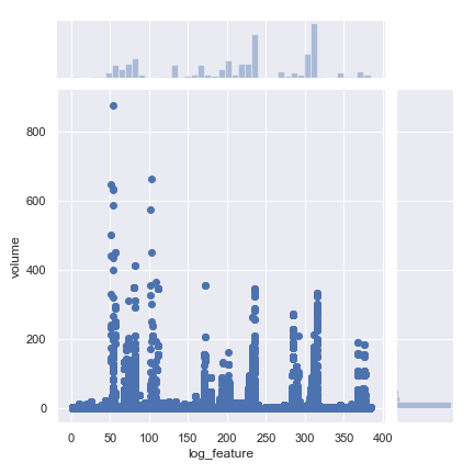
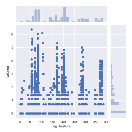
Taking the log of volume gives us a better scale, so we will be using the log transform of the ‘volume’ feature.

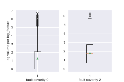
Let’s continue to look into the relationships surrounding log_feature by looking at a boxplot of how the volumes vary depending on our target: fault severity.

Lets take a look at some more graphs to try and get a sense of how the variables are related to one another.

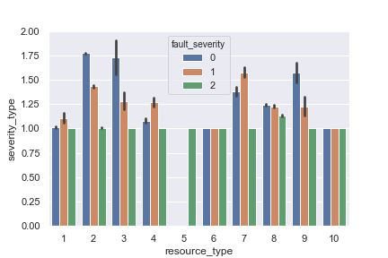
This graph shows the frequency of fault severity per resource type and severity type.

We can see that resource type 5 only has 2, or ‘critical’ fault severity. We can also see that resource types 2, 3, and 9 have higher chance of 0 fault severity.

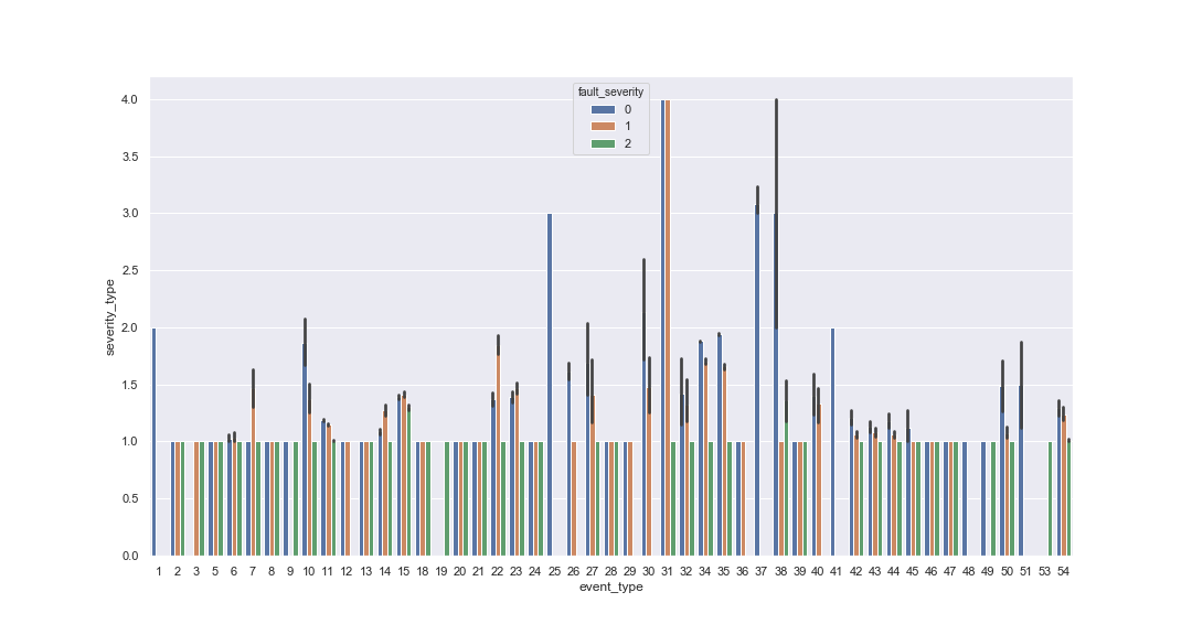
We can see some relationships within each event type or resource type, but no real overarching trends. This is why we have models to pick up on the more subtle relationships between variables.

Lets prepare our data for the model by getting dummies on our object columns. After that, we will group our data by ID number, since we want to look at the fault severity at each ID.

data = data.groupby('id', sort = False).sum()

First, we convert resource_type, severity_type, event_type, and log_feature to string values and use pd.getdummies on them, since we dont want our model to infer direction from different values (resource_type 2 is not higher than 1).

We then separate the feature and target variables, and randomly select training and test rows by using sklearn’s train_test_split. We then decide to use the gradient boosting classifier to predict to fit to our data and predict.

#The Gradient Boosting Classifier fits our data the best
gbc_model = gbc.fit(x_train, y_train)

gbc_accuracy = accuracy_score(y_train, gbc.predict(x_train))
print(gbc_accuracy)


#setting up prediction probabilities for each row
y_pred_proba = gbc.predict_proba(x_test)
y_pred = gbc.predict(x_test)

After predicting the probability, we want to create an output that is easily readable by our supervisor so that they can send the service techs to the correct locations.

#Make a DataFrame of the predictions
result = pd.DataFrame({
    "id": x_test.index,
    "Predicted fault_severity": y_pred,
    "prediction_probability_0": y_pred_proba[:, 0],
    "prediction_probability_1": y_pred_proba[:, 1],
    "prediction_probability_2": y_pred_proba[:, 2]},
    columns =['id', 'Predicted fault_severity', "prediction_probability_0",
              "prediction_probability_1", "prediction_probability_2"])

result.head(10)

Next, we sort the values by most likely to have a severe fault.

result.sort_values(['prediction_probability_2'], ascending= False, inplace= True)
result.head(20)'

After we get this table, all we need to do is write it to a csv and send it to our boss so the service techs can do their thing!

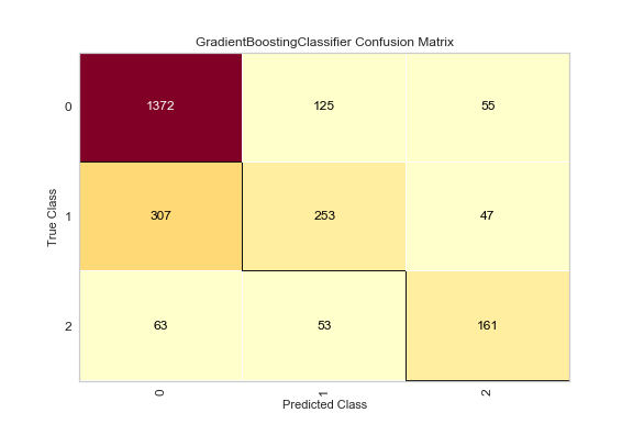
Our predictions with the basic model are decent, but as you can see in the confusion matrix below, there is only a 58% chance that we will predict a fault severity of 2 correctly.

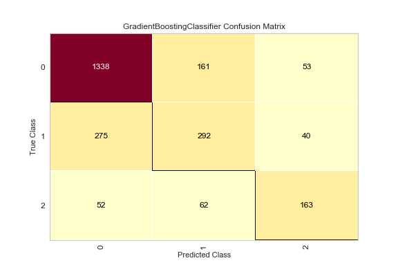
After some hyperparameter tuning, we can increase this to 63% chance that a 2 is predicted correctly, and nearly 80% chance there is at least a minor issue with the site. Given that the assignment is to give insight into a technician’s first assignment of the day, 63% is a considerable increase to chance for very low risk.

Basic GBC Model:

Parameter Tuned GBC:

Graphs made by using matplotlib, seaborn, and yellowbrick.

Link to Jupyter notebook may be coming soon here, or can be sent upon request.